Understanding Mutual Information

For this post I hope to accomplish a few different things. I will review a brilliant document put together by Erik G. Learned-Miller. I found this document when attempting to better understand the concept of ‘Mutual Information’, and it has been by far the most influential document in my understanding of entropy and mutual information. It is a short document, only 3 pages, with the purpose of being an introduction to entropy and mutual information for discrete random variables. Erik does something that I think so many teachers miss when introducing students to new concepts, which is using real-world, easy to understand examples to aid with the formulas. I hope I can add some intuition behind what entropy, joint entropy, and mutual information actually represent, as well as review some simple and more complex examples that I am currently working on in my research.

Entropy

When I started to dig into what mutual information really represents, a certain word kept popping up: Entropy. Now I heard about entropy way back in highschool chemistry and physics but I’ll be perfectly honest; I had no real understanding of the term, especially since I couldn’t see how it could seemingly be so related to every field of science. So, what does entropy mean?

Entropy refers to the amount of uncertainty that an event has. If an event A has multiple outcomes, and you have no idea which outcome will occur, the event A has high entropy. For example, if you roll a fair 6-sided die, this event has a high entropy because each number is equally likely to appear during the roll. If event B has multiple outcomes, and you are very certain about the outcome, the event has low entropy. For example, if event is whether or not the sun will come up tomorrow, this event (hopefully) has a low entropy, since we are confident that the sun will come up tomorrow morning.

As Erik points out in his document, entropy is a function of two things: 1) the number of possible outcomes, and 2) the frequency (probability) of each outcome. Erik gives very good intuition when he says:

Consider a random variable X representing the number that comes up on a roulette wheel and a random variable Y representing the number that comes up on a fair 6-sided die. The entropy of X is greater than the entropy of Y. In addition to the numbers 1 through 6, the values on the roulette wheel can take on the values 7 through 36. In some sense, it is less predictable.

On top of this, if the roullete wheel is rigged to always come up as 15 lets say, then since the probability of it landing on 15 is 100%, the entropy is very low. To formalize the entropy of a discrete random variable $X$ that takes on the values in the set $\mathcal{X} = {x_1, x_2, …, x_n}$ and is definied by a probability distribution $P(X)$, we can write:

\begin{equation} H(X)=-\sum_{x\in \mathcal{X}}P(x)logP(x) \end{equation}

Where $H(X)$ is the entropy of the random variable $X$. One interesting tidbit Erik throws in there is that there are different units to represent entropy in. The entropy is expressed in bits if the log has a base of 2, but is expressed in nats if the log has a base of 10. I personally like the sound of nats more, but bits is by far more commonly used.

Joint Entropy

The next thing to understand, when the end goal is to understand mutual information, is the intuition behind joint entropy. Now joint entropy is very similar to entropy, except that joint entropy is the entropy of two events occuring. We again denote these events as random variables $X$ and $Y$ and the question “what is the joint entropy of $X$ and $Y$?” can be understood as “how uncertain are we about the outcome of events $X$ and $Y$ when they both occur?”. Not surprisingly, the equation is the same as the equation for entropy, except the summation is over both random variables.

\begin{equation} H(X)=-\sum_{y \in \mathcal{Y}}\sum_{x\in \mathcal{X}}P(x)logP(x) \end{equation}

One thing that helps me understand some of the intuition behind these equations is viewing it as an expectation (basically a weighted average). You know when you calculate grades for a class? You take the sum of the grades you have, multiplied by the weight of each grade, right? Well its exact same for entropy and joint entropy, except the ‘grades’ are the uncertainty (or information content) and the weighting of each uncertainty value is the probability of that(those) specific event(s) occuring, summed over all possible events.

Mutual Information

On a high level, mutual information is a value that quantifies how much information knowing one random variable gives you about another when they are sampled simultaneously. An important theory of information theory is that the mutual information of two random variables is 0 if and only if they are statistically independant. For example, if $X$ represents the value of spinning a roulette wheel, and $Y$ represents the value of spinning a different roulette wheel, the mutual information between $X$ and $Y$ is 0. However if $X$ represents the color of the roulette wheel, and $Y$ represents the number, then they share some mutual information, as only certain numbers are found on certain colors of the roulette wheel. To formalize the definition of mutual information of random variables $X$ and $Y$,

\begin{equation} I(X ; Y)=\sum_{x \in \mathcal{X}} \sum_{y \in \mathcal{Y}} P(x, y) \log \frac{P(x, y)}{P(x) P(y)} \end{equation}

Similar to the intuition as before, we can understand this equation as the expectation of shared information between random variables $X$ and $Y$. $P(x, y)$ is the weighting while $\log \frac{P(x, y)}{P(x) P(y)}$ is the mutual information for an individual outcome. The mutual information for an individual outcome can be understood to be measuring the difference ($\log$) between the two sampled random variables, $x$ and $y$, if they are statistically dependant ($P(x, y)$) compared to if they are statistically independant ($P(x) P(y)$). Then, to calculate the total mutual information, we just sum over all possible events: $\sum_{x \in \mathcal{X}} \sum_{y \in \mathcal{Y}}$

Application: Information Invariant Clustering

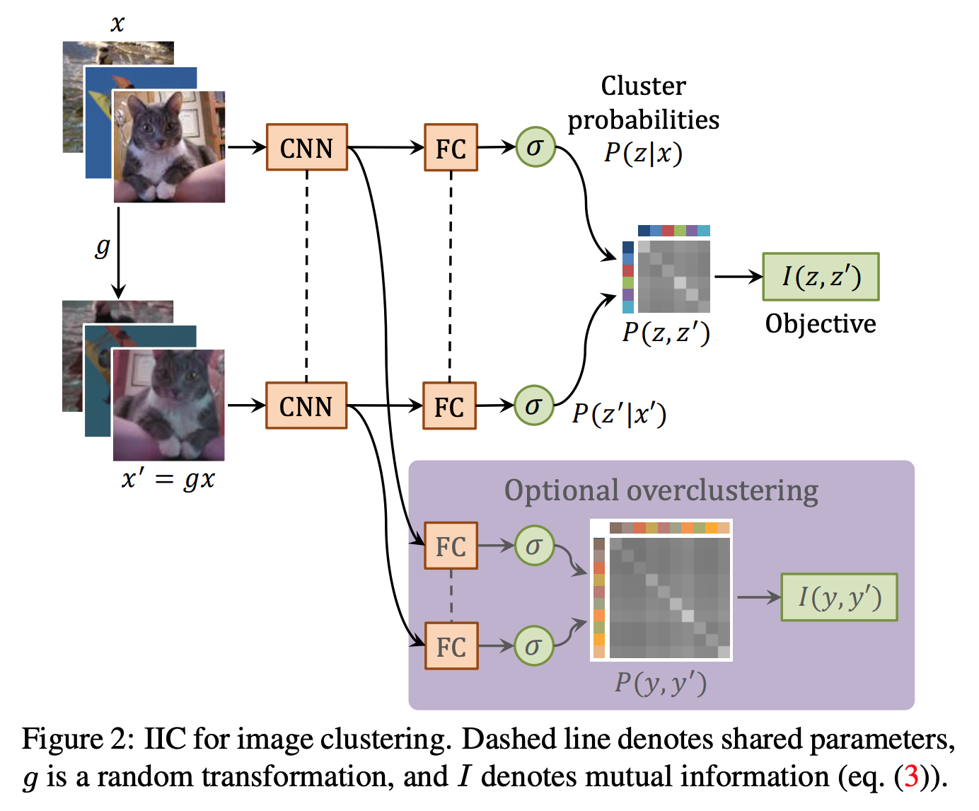
In a recent ICCV 2019 paper, the authors used mutual information as a learning objective for the task of unsupervised image clustering. What I really liked about this work was the simplicity of the implementation, with the code to calculate mutual information being only a few lines or so. Specifically, they feed an image through a neural network twice, once with the normal image, and once with a transformation applied (e.g. hue, saturation, brightness, rotation, etc.). They can then take the two outputs of the neural network, which are in the format of softmax probability distributions. They then calculate the joint probability distribution by multiplying the softmax distributions together (one transposed) which takes the form of:

\begin{equation} P=\frac{1}{n} \sum_{i=1}^{n} \Phi\left(x_{i} \right) \cdot \Phi\left(x_{i}^{\prime}\right)^{\top} \end{equation}

where $\Phi$ is the neural network, $x_{i}$ is the initial image, $x_{i}^{\prime}$ is the transformed image, and $n$ is the number of dataset examples. Then to calculate the mutual information, you just use the mutual information equation:

\begin{equation} I\left(z, z^{\prime}\right)=I(P)=\sum_{c=1}^{C} \sum_{c^{\prime}=1}^{C} P_{c c^{\prime}} \cdot \ln \frac{P_{c c^{\prime}}}{P_{c} \cdot P_{c^{\prime}}} \end{equation}

where $c$ is the class of the first image, $c^{\prime}$ is the class of the second image, and $C$ is the number of classes (i.e. the length of the softmax distribution). Here is a good diagram they have in the paper to visualize the process (the overclustering head is just a way to make use of extra unlabelled data):

In my own work, I am attempting to implement information invariant clustering for the task of unsupervised video clustering. The interesting thing seems to be how to use the temporal dimension during the transformation process. I.e. do we just take random samples of the same video? Or should we constrain the starting frame to be near the original videos starting frame so the network can learn to distill more information? We will see as I will be running some experiments over the next few weeks to explore this idea.

Conclusions

We can really view joint entropy and mutual information as expectations (i.e. basically a weighted average) measuring information and information sharing between random variables. We also got to see a really interesting application of mutual information being used for the task of unsupervised image clustering, where the tractability of mutual information stems from treating the softmax output of the network as a probability distribution in the calculations.

I hope helped some of you gain a better intuition behind what entropy, joint entropy, and mutual information is. See you next time and keep learning :) .